31.2 Euler’s Method
AHL 5.18
- how Euler’s method builds an approximate solution of \(\dfrac{\mathrm{d}y}{\mathrm{d}x} = f(x, y)\) step by step
- how to set out the working in a table
- how the step size \(h\) affects the accuracy, and why an estimate can be too big or too small
- how to do the calculation with a spreadsheet on the TI-Nspire CX II
Many differential equations cannot be solved exactly. Euler’s method gives a numerical answer instead.
The idea of Euler’s method
We want the solution of \(\dfrac{\mathrm{d}y}{\mathrm{d}x} = f(x, y)\) through a known point \((x_0, y_0)\). We do not know the curve, but the DE tells us its gradient at any point.
- Choose a small step size \(h\). The \(x\)-values are \(x_1 = x_0 + h\), \(x_2 = x_1 + h\), and so on.
- At \((x_0, y_0)\) the gradient is \(f(x_0, y_0)\). Follow the tangent for a horizontal distance \(h\). The rise is \(h \times f(x_0, y_0)\), so we arrive at \(y_1 = y_0 + h\,f(x_0, y_0)\).
- At the new point, recalculate the gradient and take another step. Repeat.
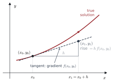
Euler’s method In the HL formula booklet
\[ y_{n+1} = y_n + h \times f(x_n, y_n) ; \qquad x_{n+1} = x_n + h , \]
- \(y_n\): the estimate of \(y\) at \(x = x_n\) (\(y_0\) comes from the initial condition)
- \(h\): a constant, the step length
- \(f(x_n, y_n)\): the gradient \(\dfrac{\mathrm{d}y}{\mathrm{d}x} = f(x, y)\) at the point \((x_n, y_n)\)
- \(x_n\): the \(x\)-value after \(n\) steps
The points \((x_0, y_0), (x_1, y_1), (x_2, y_2), \ldots\) are joined by straight segments. This “polygon” is an approximation to the solution curve (Figure 2). After each step the direction is corrected, because the gradient is recalculated.
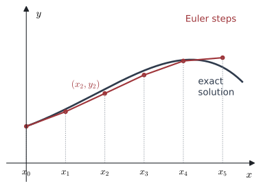
Accuracy
- A smaller step size \(h\) usually gives a better estimate, but needs more steps.
- If the solution curve is concave up, the tangent lies below the curve, so Euler’s method underestimates. If the curve is concave down, it overestimates.
Link with the Fundamental Theorem of Calculus. If \(\dfrac{\mathrm{d}y}{\mathrm{d}x} = f(x)\) only, then \(y_n = y_0 + h f(x_0) + h f(x_1) + \cdots + h f(x_{n-1})\), which is a sum of rectangle areas. If we use infinitely many steps (\(n \to \infty\), \(h \to 0\)) to reach \(x = b\), the sum becomes an integral:
\[ y(b) = y(x_0) + \int_{x_0}^{b} \frac{\mathrm{d}y}{\mathrm{d}x}\,\mathrm{d}x . \]
Example 1 Consider the differential equation \(\dfrac{\mathrm{d}y}{\mathrm{d}x} = 4\mathrm{e}^{-2x} + 1\) with \(y(0) = 1\).
(a) Use Euler’s method to estimate \(y(0.4)\) with
\(\quad\) (i) \(h = 0.2\) (two steps), \(\qquad\) (ii) \(h = 0.1\) (four steps).
(b) Find \(y(0.4)\) exactly, using the Fundamental Theorem of Calculus. Comment on your results.
Let \(f(x) = 4\mathrm{e}^{-2x} + 1\).
(a)(i) \(h = 0.2\):
| \(n\) | \(x_n\) | \(y_n\) | \(f(x_n)\) | \(y_{n+1} = y_n + 0.2 f(x_n)\) |
|---|---|---|---|---|
| 0 | 0 | 1 | 5 | 2 |
| 1 | 0.2 | 2 | 3.681,28 | 2.736,26 |
\(y(0.4) \approx 2.74\).
(ii) \(h = 0.1\):
| \(n\) | \(x_n\) | \(y_n\) | \(f(x_n)\) | \(y_{n+1} = y_n + 0.1 f(x_n)\) |
|---|---|---|---|---|
| 0 | 0 | 1 | 5 | 1.5 |
| 1 | 0.1 | 1.5 | 4.274,92 | 1.927,49 |
| 2 | 0.2 | 1.927,49 | 3.681,28 | 2.295,62 |
| 3 | 0.3 | 2.295,62 | 3.195,25 | 2.615,14 |
\(y(0.4) \approx 2.62\).
(b) \(y(0.4) = 1 + \displaystyle\int_0^{0.4} (4\mathrm{e}^{-2x} + 1)\,\mathrm{d}x = 1 + \Big[-2\mathrm{e}^{-2x} + x\Big]_0^{0.4} = 1 + (-2\mathrm{e}^{-0.8} + 0.4) - (-2) = 3.4 - 2\mathrm{e}^{-0.8}\).
\(y(0.4) = 2.501\) (4 s.f.).
Comment. Both estimates are too large, because \(\dfrac{\mathrm{d}^2y}{\mathrm{d}x^2} = -8\mathrm{e}^{-2x} < 0\): the curve is concave down, so each tangent step goes above the curve. The smaller step \(h = 0.1\) gives the better estimate (error about \(0.11\) instead of \(0.23\)).
Example 2 Consider the differential equation \(\dfrac{\mathrm{d}y}{\mathrm{d}x} = y - x^2\) with initial point \((0, 1)\).
(a) Use Euler’s method with step size \(h = 0.1\) to complete the table and estimate \(y(0.5)\).
| Step | \(x_{n-1}\) | \(y_{n-1}\) | \(\dfrac{\mathrm{d}y}{\mathrm{d}x}\) | \(x_n\) | \(y_n\) |
|---|---|---|---|---|---|
| 1 | 0 | 1 | 1 | 0.1 | 1.1 |
| 2 | 0.1 | 1.1 | |||
| 3 | |||||
| 4 | |||||
| 5 |
(b) Plot the approximate solution for \(0 \le x \le 0.5\).
(a) At each step: gradient \(= y_{n-1} - x_{n-1}^2\), then \(y_n = y_{n-1} + 0.1 \times \text{gradient}\).
| Step | \(x_{n-1}\) | \(y_{n-1}\) | \(\dfrac{\mathrm{d}y}{\mathrm{d}x}\) | \(x_n\) | \(y_n\) |
|---|---|---|---|---|---|
| 1 | 0 | 1 | 1 | 0.1 | 1.1 |
| 2 | 0.1 | 1.1 | 1.09 | 0.2 | 1.209 |
| 3 | 0.2 | 1.209 | 1.169 | 0.3 | 1.3259 |
| 4 | 0.3 | 1.3259 | 1.2359 | 0.4 | 1.449,49 |
| 5 | 0.4 | 1.449,49 | 1.289,49 | 0.5 | 1.578,44 |
\(y(0.5) \approx 1.58\).
(b) Plot the points \((0, 1), (0.1, 1.1), (0.2, 1.209), (0.3, 1.326), (0.4, 1.449), (0.5, 1.578)\) and join them with straight segments. The result looks like the left part of Figure 2, but with smaller steps.
(In Section 31.5 you can solve this DE exactly: \(y = x^2 + 2x + 2 - \mathrm{e}^x\), so \(y(0.5) = 1.601\). Here the curve is concave up near \(x = 0\), so Euler’s method underestimates.)
Use a Lists & Spreadsheet page. For Example 2 (\(h = 0.1\), \(f(x, y) = y - x^2\), start \((0, 1)\)):
- Cell A1: type
0. Cell B1: type1. - Cell A2: type
=a1+0.1. - Cell B2: type
=b1+0.1*(b1-a1^2)(this is \(y_n = y_{n-1} + h f(x_{n-1}, y_{n-1})\)). - Select cells A2 and B2, then Menu → Data → Fill, press the down arrow until you reach row 6, and press enter.
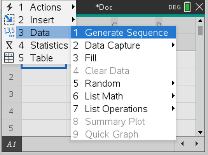
Row 6 shows \(x = 0.5\) and \(y \approx 1.578\,44\). To change the step size or the DE, edit row 2 and fill down again. For Example 1 use =b1+0.1*(4*e^(-2*a1)+1) in B2.
Common errors
| ✗ Wrong | ✓ Right | Why |
|---|---|---|
| Using the new point to find the gradient for the same step | Gradient at the start of each step: \(f(x_n, y_n)\) | Euler’s method follows the tangent from the known point. |
| Forgetting to multiply by \(h\) | \(y_{n+1} = y_n + h f(x_n, y_n)\) | The gradient is a rate; the change in \(y\) is gradient \(\times\) step. |
| Counting the steps wrongly | Number of steps \(= \dfrac{b - x_0}{h}\) | From \(x = 1\) to \(x = 1.5\) with \(h = 0.1\) is 5 steps. |
| Rounding heavily at every step | Keep full accuracy (or use the GDC) | Rounding errors add up over many steps. |
| “Euler’s method always underestimates” | It depends on the concavity | Concave up: under; concave down: over. |
Exercises
1 Use Euler’s method with \(h = 0.1\) to estimate \(y(0.3)\) for \(\dfrac{\mathrm{d}y}{\mathrm{d}x} = x + y\), \(y(0) = 1\).
\(y_1 = 1 + 0.1(0 + 1) = 1.1\); \(\;y_2 = 1.1 + 0.1(0.1 + 1.1) = 1.22\); \(\;y_3 = 1.22 + 0.1(0.2 + 1.22) = 1.362\).
\(y(0.3) \approx 1.362\).
2 For \(\dfrac{\mathrm{d}y}{\mathrm{d}x} = x + y\) with step size \(h = 0.1\), show that Euler’s method gives \(y_{n+1} = 1.1\,y_n + 0.1\,x_n\).
\(y_{n+1} = y_n + 0.1(x_n + y_n) = y_n + 0.1x_n + 0.1y_n = 1.1y_n + 0.1x_n\).
3 A curve passes through the point \((1, 3)\) and satisfies \(\dfrac{\mathrm{d}y}{\mathrm{d}x} = 2x - y\). Use Euler’s method with step size \(0.1\) to estimate \(y\) when \(x = 1.5\).
Five steps:
| \(x_n\) | 1 | 1.1 | 1.2 | 1.3 | 1.4 | 1.5 |
|---|---|---|---|---|---|---|
| \(y_n\) | 3 | 2.9 | 2.83 | 2.787 | 2.7683 | 2.771,47 |
| \(2x_n - y_n\) | \(-1\) | \(-0.7\) | \(-0.43\) | \(-0.187\) | \(0.0317\) |
\(y(1.5) \approx 2.77\).
4 The function \(y\) satisfies \(\dfrac{\mathrm{d}y}{\mathrm{d}x} = 3x^2\) and \(y(0) = 0\).
(a) Use Euler’s method with \(h = 0.5\) to estimate \(y(1)\).
(b) Find the exact value of \(y(1)\), and explain why the estimate is too small.
(a) \(y_1 = 0 + 0.5(0) = 0\); \(\;y_2 = 0 + 0.5(3 \times 0.25) = 0.375\). \(\;y(1) \approx 0.375\).
(b) \(y = x^3\), so \(y(1) = 1\). The curve \(y = x^3\) is concave up for \(x > 0\), so each tangent step stays below the curve.
5 Consider \(\dfrac{\mathrm{d}y}{\mathrm{d}x} = \dfrac{1}{1 + x}\), \(y(0) = 0\).
(a) Estimate \(y(1)\) using Euler’s method with \(h = 0.5\), and then with \(h = 0.25\).
(b) Find the exact value of \(y(1)\) and the percentage error of each estimate.
(a) \(h = 0.5\): \(y_1 = 0.5\), \(y_2 = 0.5 + 0.5 \times \frac{1}{1.5} = 0.8333\).
\(h = 0.25\): \(0.25,\ 0.25 + 0.2 = 0.45,\ 0.45 + 0.166\,67 = 0.616\,67,\ 0.616\,67 + 0.142\,86 = 0.7595\).
(b) \(y(1) = \displaystyle\int_0^1 \frac{1}{1 + x}\,\mathrm{d}x = \ln 2 = 0.6931\).
Errors: \(\dfrac{0.8333 - 0.6931}{0.6931} \times 100 = 20.2\%\) and \(\dfrac{0.7595 - 0.6931}{0.6931} \times 100 = 9.58\%\). Halving \(h\) roughly halves the error.
6 The function \(y\) satisfies \(\dfrac{\mathrm{d}y}{\mathrm{d}x} = \dfrac{2x}{y}\), \(y(1) = 2\).
(a) Use Euler’s method with \(h = 0.25\) to estimate \(y(1.5)\).
(b) Given that the exact solution is \(y = \sqrt{2x^2 + 2}\), find the error.
(a) \(y_1 = 2 + 0.25 \times \dfrac{2}{2} = 2.25\); \(\;y_2 = 2.25 + 0.25 \times \dfrac{2.5}{2.25} = 2.5278\).
(b) \(y(1.5) = \sqrt{6.5} = 2.5495\). Error \(= 2.5495 - 2.5278 = 0.0217\) (an underestimate).
7 Consider \(\dfrac{\mathrm{d}y}{\mathrm{d}x} = y\), \(y(0) = 1\), whose exact solution is \(y = \mathrm{e}^x\).
(a) Use Euler’s method with \(h = 0.25\) to estimate \(y(1)\).
(b) Show that with \(n\) equal steps from \(x = 0\) to \(x = 1\) the estimate is \(\left(1 + \dfrac{1}{n}\right)^n\). What happens as \(n \to \infty\)?
(a) Each step multiplies \(y\) by \(1.25\): \(\;y(1) \approx 1.25^4 = 2.4414\).
(b) \(h = \dfrac{1}{n}\) and \(y_{k+1} = y_k + h y_k = \left(1 + \dfrac{1}{n}\right) y_k\). After \(n\) steps \(y_n = \left(1 + \dfrac{1}{n}\right)^n\). As \(n \to \infty\) this tends to \(\mathrm{e} = 2.718\ldots\), the exact value.
8 Use Euler’s method with \(h = 0.2\) to estimate \(y(1)\) for \(\dfrac{\mathrm{d}y}{\mathrm{d}x} = x - y^2\), \(y(0) = 1\). Give the answer to 3 significant figures.
| \(x_n\) | 0 | 0.2 | 0.4 | 0.6 | 0.8 | 1 |
|---|---|---|---|---|---|---|
| \(y_n\) | 1 | 0.8 | 0.712 | 0.690,61 | 0.715,22 | 0.772,91 |
\(y(1) \approx 0.773\).
9 Use Euler’s method with \(h = 0.2\) to estimate \(y(1)\) for \(\dfrac{\mathrm{d}y}{\mathrm{d}x} = x^2 + y^2\), \(y(0) = 0\).
| \(x_n\) | 0 | 0.2 | 0.4 | 0.6 | 0.8 | 1 |
|---|---|---|---|---|---|---|
| \(y_n\) | 0 | 0 | 0.008 | 0.040,01 | 0.112,33 | 0.242,86 |
\(y(1) \approx 0.243\).
10 A population of birds \(P\) on an island is modelled by \(\dfrac{\mathrm{d}P}{\mathrm{d}t} = 0.3P\left(1 - \dfrac{P}{200}\right)\), where \(t\) is the time in years and \(P(0) = 20\). Use Euler’s method with a step of 1 year to estimate the population after 5 years.
| \(t\) | 0 | 1 | 2 | 3 | 4 | 5 |
|---|---|---|---|---|---|---|
| \(P\) | 20 | 25.4 | 32.052 | 40.127 | 49.750 | 60.962 |
About 61 birds after 5 years.