19.1 Continuous Random Variables
AHL 4.14
- the difference between a discrete and a continuous random variable
- what a probability density function (p.d.f.) \(f(x)\) is, and why \(\displaystyle\int_{-\infty}^{\infty} f(x)\,\mathrm{d}x = 1\)
- how to find probabilities as areas under \(y = f(x)\), using definite integrals
- why \(\mathrm{P}(X = a) = 0\) for a continuous random variable
- how to find the expected value \(\mathrm{E}(X)\), and \(\mathrm{E}\big(g(X)\big)\), and the rules \(\mathrm{E}(aX + b) = a\,\mathrm{E}(X) + b\)
This section uses definite integrals. See Unit 28 for the idea of a definite integral as an area.
Discrete and continuous random variables
In Unit 18 we met discrete random variables. They take values that we can list, for example \(0, 1, 2, 3, \ldots\) (a binomial variable is an example).
A continuous random variable is different. We cannot list its values, but we can describe the range of its values.
| Continuous random variable | Possible range of values |
|---|---|
| The time taken by a student to run 100 m | 11 s to 18 s |
| The mass of an apple from one farm | 120 g to 230 g |
| The lifetime of a phone charger | 1 year to 6 years |
These are measurements. The number of different values we can record depends only on how accurate our measuring instrument is. A continuous random variable can take infinitely many values, so the probability of any single value is zero. Instead, we give probabilities to intervals of values.
As a rule of thumb:
- measurements of length, time, mass, temperature, … are continuous;
- counts (the number of goals, the number of heads, …) are discrete.
Continuous random variable Not in the formula booklet
A random variable \(X\) is continuous if it can take all values in one or more intervals of the real number line.
Probability density functions
A continuous random variable has too many values to list in a table, so we describe its probabilities with a function \(f(x)\) and its graph. This function is called the probability density function, or p.d.f. for short (plural: p.d.f.s). The probability that \(X\) lies between \(a\) and \(b\) is the area under the graph from \(x = a\) to \(x = b\).
Probability density function (p.d.f.) Not in the formula booklet
The probability density function of a continuous random variable \(X\) is a function \(f(x)\) with
- \(f(x) \geq 0\) for all \(x \in \mathbb{R}\)
- \(\displaystyle\int_{-\infty}^{\infty} f(x)\,\mathrm{d}x = 1\) \(\quad\) (the total area under the curve is \(1\))
- \(\displaystyle\mathrm{P}(a \leq X \leq b) = \int_a^b f(x)\,\mathrm{d}x\) \(\quad\) (probability \(=\) area between \(x = a\) and \(x = b\))
- \(X\): a continuous random variable
- \(f(x)\): the probability density function (p.d.f.) of \(X\)
- \(a\), \(b\): the ends of an interval (\(a \leq b\))
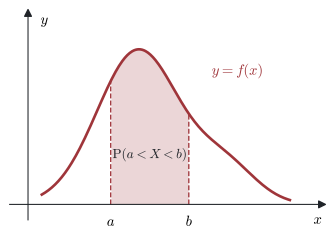
Often \(f(x)\) is non-zero only on an interval, for example \(0 \leq x \leq 2\), and \(f(x) = 0\) “otherwise”. Then the integral from \(-\infty\) to \(\infty\) is just the integral over that interval. The syllabus also includes piecewise p.d.f.s, which use different formulae on different intervals. Then you split the integral into parts.
Single values have probability zero
For a discrete random variable, \(\mathrm{P}(X = a) \neq 0\) for some numbers \(a\). For a continuous random variable, the “area” above a single point is a line, with width zero:
\[ \mathrm{P}(X = a) = \int_a^a f(x)\,\mathrm{d}x = 0 \qquad \text{for every } a \in \mathbb{R} . \]
So for a continuous random variable it does not matter whether we use \(<\) or \(\leq\):
\[ \mathrm{P}(a \leq X \leq b) = \mathrm{P}(a < X \leq b) = \mathrm{P}(a \leq X < b) = \mathrm{P}(a < X < b) . \]
(This is not true for discrete random variables.)
Example 1 A continuous random variable \(X\) has probability density function
\[ f(x) = \begin{cases} kx^3, & 0 < x < 2 \\ 0, & \text{otherwise.} \end{cases} \]
(a) Find the value of the constant \(k\).
(b) Find \(\mathrm{P}(1 \leq X \leq 1.5)\).
(c) Find \(\mathrm{P}(X > 1 \mid X < 1.5)\).
(a) The total area is \(1\):
\[ \int_0^2 kx^3\,\mathrm{d}x = k\left[\frac{x^4}{4}\right]_0^2 = k \times \frac{16}{4} = 4k = 1 \;\Longrightarrow\; k = \frac{1}{4} . \]
(b)
\[ \mathrm{P}(1 \leq X \leq 1.5) = \int_1^{1.5} \frac{x^3}{4}\,\mathrm{d}x = \left[\frac{x^4}{16}\right]_1^{1.5} = \frac{1}{16}\left(\frac{81}{16} - 1\right) = \frac{65}{256} \;(\approx 0.254) . \]
(c) Use conditional probability, \(\mathrm{P}(A \mid B) = \dfrac{\mathrm{P}(A \cap B)}{\mathrm{P}(B)}\). “\(X > 1\) and \(X < 1.5\)” means \(1 < X < 1.5\).
\[ \mathrm{P}(X < 1.5) = \left[\frac{x^4}{16}\right]_0^{1.5} = \frac{81}{256}, \qquad \mathrm{P}(X > 1 \mid X < 1.5) = \frac{\mathrm{P}(1 < X < 1.5)}{\mathrm{P}(X < 1.5)} = \dfrac{\;\frac{65}{256}\;}{\;\frac{81}{256}\;} = \frac{65}{81} . \]
Example 2 A continuous random variable \(X\) has probability density function
\[ f(x) = \begin{cases} kx, & 0 \leq x \leq 1 \\[2pt] \dfrac{k}{2}(3 - x), & 1 \leq x \leq 3 \\[2pt] 0, & \text{otherwise.} \end{cases} \]
(a) Find the value of the constant \(k\).
(b) Find the value of \(a\) such that \(\mathrm{P}(X > a) = 0.06\).
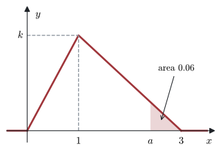
(a) The graph is a triangle with base \(3\) and height \(k\) (see Figure 2). Its area is \(1\):
\[ \frac{1}{2} \times 3 \times k = 1 \;\Longrightarrow\; k = \frac{2}{3} . \]
(By integration: \(\displaystyle\int_0^1 kx\,\mathrm{d}x + \int_1^3 \frac{k}{2}(3 - x)\,\mathrm{d}x = \frac{k}{2} + k = \frac{3k}{2} = 1\).)
(b) \(\mathrm{P}(X > 1) = 1 - \dfrac{1}{2} \times 1 \times \dfrac{2}{3} = \dfrac{2}{3}\), which is more than \(0.06\). So \(a\) is between \(1\) and \(3\), and \(f(x) = \dfrac{1}{3}(3 - x)\) there.
\[ \mathrm{P}(X > a) = \int_a^3 \frac{1}{3}(3 - x)\,\mathrm{d}x = \left[-\frac{(3 - x)^2}{6}\right]_a^3 = \frac{(3 - a)^2}{6} . \]
\[ \frac{(3 - a)^2}{6} = 0.06 \;\Longrightarrow\; (3 - a)^2 = 0.36 \;\Longrightarrow\; 3 - a = 0.6 \;\Longrightarrow\; a = 2.4 . \]
(We take \(3 - a = +0.6\) because \(a < 3\).)
Calculator page → Menu → Calculus → Numerical Integral. Fill in the template, for example \(\displaystyle\int_{1}^{1.5} \frac{x^3}{4}\,\mathrm{d}x\), and press enter. You get \(0.253906\ldots\)
To find an unknown limit (like \(a\) in Example 2), use Menu → Algebra → Numerical Solve, for example nSolve( \(\displaystyle\int_a^3 \frac{1}{3}(3 - x)\,\mathrm{d}x = 0.06,\ a\) ) with a starting value between \(1\) and \(3\).
Expectation of a continuous random variable
For a discrete random variable, \(\mathrm{E}(X) = \sum x\,\mathrm{P}(X = x)\). For a continuous random variable the sum becomes an integral, and \(\mathrm{P}(X = x)\) is replaced by \(f(x)\).
Expected value (mean) of a continuous random variable In the HL formula booklet
\[ \mathrm{E}(X) = \mu = \int_{-\infty}^{\infty} x\,f(x)\,\mathrm{d}x \]
- \(\mathrm{E}(X)\), \(\mu\): the expected value (mean) of \(X\)
- \(x\): a value of \(X\) (the variable of integration)
- \(f(x)\): the p.d.f. of \(X\)
\(\mathrm{E}(X)\) is also written \(\mu\), and is called the mean of \(X\).
The limits are \(-\infty\) and \(\infty\), but \(f(x) = 0\) outside the interval where the p.d.f. is defined, so in practice you integrate \(x\,f(x)\) only over that interval (for example, from \(0\) to \(2\) if \(f(x)\) is non-zero only for \(0 \le x \le 2\)).
Example 3 A continuous random variable \(X\) has probability density function
\[ f(x) = \begin{cases} \dfrac{3}{32}(x - 1)(5 - x), & 1 \leq x \leq 5 \\[2pt] 0, & \text{otherwise.} \end{cases} \]
Find \(\mathrm{E}(X)\).
Expand first: \(x(x - 1)(5 - x) = x(-x^2 + 6x - 5) = -x^3 + 6x^2 - 5x\).
\[ \begin{aligned} \mathrm{E}(X) &= \frac{3}{32}\int_1^5 \left(-x^3 + 6x^2 - 5x\right)\mathrm{d}x = \frac{3}{32}\left[-\frac{x^4}{4} + 2x^3 - \frac{5x^2}{2}\right]_1^5 \\ &= \frac{3}{32}\left(\frac{125}{4} - \left(-\frac{3}{4}\right)\right) \\ &= \frac{3}{32} \times 32 \\ &= 3 . \end{aligned} \]
Symmetry Not in the formula booklet
If the graph of \(y = f(x)\) is symmetrical about the line \(x = c\), then \(\mathrm{E}(X) = c\).
- \(f(x)\): the p.d.f. of \(X\)
- \(c\): a constant; \(x = c\) is the line of symmetry
In Example 3, \(y = f(x)\) is a parabola with roots \(1\) and \(5\), so it is symmetrical about \(x = 3\). We could simply write down \(\mathrm{E}(X) = 3\).
The expected value of a function of \(X\)
Expected value of \(g(X)\) Not in the formula booklet
If \(X\) has p.d.f. \(f(x)\) and \(g\) is any function, then
\[ \mathrm{E}\big(g(X)\big) = \int_{-\infty}^{\infty} g(x)\,f(x)\,\mathrm{d}x . \]
For example, \(\displaystyle\mathrm{E}(X^2) = \int_{-\infty}^{\infty} x^2 f(x)\,\mathrm{d}x\) and \(\displaystyle\mathrm{E}\big(\sqrt{X}\big) = \int_{-\infty}^{\infty} \sqrt{x}\,f(x)\,\mathrm{d}x\).
Note: \(\mathrm{E}(X^2)\) is not the same as \(\big(\mathrm{E}(X)\big)^2\). We will use both in Section 19.2.
Rules for expectation
Rules for expectation Partly in the HL formula booklet
For a random variable \(X\) and constants \(a\) and \(b\):
(a) \(\mathrm{E}(a) = a\)
(b) \(\mathrm{E}(aX) = a\,\mathrm{E}(X)\)
(c) \(\mathrm{E}(aX + b) = a\,\mathrm{E}(X) + b\) In the HL booklet
(d) \(\mathrm{E}\big(g(X) \pm h(X)\big) = \mathrm{E}\big(g(X)\big) \pm \mathrm{E}\big(h(X)\big)\)
- \(X\): a random variable
- \(a\), \(b\): constants (real numbers)
- \(g\), \(h\): any functions
These rules also work for discrete random variables.
Proof (continuous case). Each proof uses \(\displaystyle\int_{-\infty}^{\infty} f(x)\,\mathrm{d}x = 1\) and \(\displaystyle\int_{-\infty}^{\infty} x f(x)\,\mathrm{d}x = \mathrm{E}(X)\).
\[ \begin{aligned} \text{(a)}\quad \mathrm{E}(a) &= \int_{-\infty}^{\infty} a\,f(x)\,\mathrm{d}x = a\int_{-\infty}^{\infty} f(x)\,\mathrm{d}x \\ &= a \times 1 \\ &= a \\ \text{(b)}\quad \mathrm{E}(aX) &= \int_{-\infty}^{\infty} ax\,f(x)\,\mathrm{d}x = a\int_{-\infty}^{\infty} x\,f(x)\,\mathrm{d}x \\ &= a\,\mathrm{E}(X) \\ \text{(c)}\quad \mathrm{E}(aX + b) &= \int_{-\infty}^{\infty} (ax + b)\,f(x)\,\mathrm{d}x \\ &= a\int_{-\infty}^{\infty} x\,f(x)\,\mathrm{d}x + b\int_{-\infty}^{\infty} f(x)\,\mathrm{d}x \\ &= a\,\mathrm{E}(X) + b \end{aligned} \]
For any two random variables \(X\) and \(Y\) (they do not need to be independent),
\[ \mathrm{E}(aX + bY) = a\,\mathrm{E}(X) + b\,\mathrm{E}(Y) . \]
Combining two random variables is not in the AA syllabus. It is useful later, for example in further statistics courses.
Common errors
| ✗ Wrong | ✓ Right | Why |
|---|---|---|
| \(\mathrm{P}(X = 2) = f(2)\) | \(\mathrm{P}(X = 2) = 0\) | For a continuous variable, probability is an area, not a height. |
| \(f(x)\) can be bigger than \(1\), so it is not a p.d.f. | \(f(x) > 1\) is allowed | Only \(f(x) \geq 0\) and total area \(= 1\) are needed. |
| Integrating over the wrong interval | Use only where \(f(x) \neq 0\); split piecewise p.d.f.s | Outside its interval, \(f(x) = 0\). |
| \(\mathrm{E}(X) = \displaystyle\int f(x)\,\mathrm{d}x\) | \(\mathrm{E}(X) = \displaystyle\int x\,f(x)\,\mathrm{d}x\) | \(\int f(x)\,\mathrm{d}x\) is always \(1\). |
| \(\mathrm{E}(X^2) = \big(\mathrm{E}(X)\big)^2\) | \(\mathrm{E}(X^2) = \displaystyle\int x^2 f(x)\,\mathrm{d}x\) | They are different in general. |
| \(\mathrm{P}(X > 1 \mid X < 1.5) = \mathrm{P}(X > 1)\) | Divide by \(\mathrm{P}(X < 1.5)\) | Conditional probability: \(\dfrac{\mathrm{P}(A \cap B)}{\mathrm{P}(B)}\). |
Exercises
1 Is each random variable discrete or continuous?
(a) The number of goals scored in a football match.
(b) The time taken to run 1 km.
(c) The mass of a newborn baby.
(d) The number of emails a person receives in one day.
(a) Discrete (a count).
(b) Continuous (a time).
(c) Continuous (a mass).
(d) Discrete (a count).
2 \(X\) has p.d.f. \(f(x) = kx\) for \(0 \leq x \leq 4\), and \(f(x) = 0\) otherwise. Find \(k\) and \(\mathrm{P}(1 < X < 3)\).
\(\displaystyle\int_0^4 kx\,\mathrm{d}x = 8k = 1\), so \(k = \dfrac{1}{8}\).
\(\mathrm{P}(1 < X < 3) = \left[\dfrac{x^2}{16}\right]_1^3 = \dfrac{9 - 1}{16} = \dfrac{1}{2}\).
3 \(X\) has p.d.f. \(f(x) = k\sqrt{x}\) for \(0 \leq x \leq 4\), and \(f(x) = 0\) otherwise. Find \(k\) and \(\mathrm{P}(X > 1)\).
\(\displaystyle\int_0^4 k x^{\frac{1}{2}}\,\mathrm{d}x = k\left[\frac{2}{3}x^{\frac{3}{2}}\right]_0^4 = \frac{16k}{3} = 1\), so \(k = \dfrac{3}{16}\).
\(\mathrm{P}(X > 1) = 1 - \mathrm{P}(X \leq 1) = 1 - \dfrac{3}{16} \times \dfrac{2}{3} = 1 - \dfrac{1}{8} = \dfrac{7}{8}\).
4 \(X\) has p.d.f. \(f(x) = \dfrac{k}{x^2}\) for \(1 \leq x \leq 4\), and \(f(x) = 0\) otherwise. Find \(k\) and \(\mathrm{P}(X < 2)\).
\(\displaystyle\int_1^4 \frac{k}{x^2}\,\mathrm{d}x = k\left[-\frac{1}{x}\right]_1^4 = k\left(1 - \frac{1}{4}\right) = \frac{3k}{4} = 1\), so \(k = \dfrac{4}{3}\).
\(\mathrm{P}(X < 2) = \dfrac{4}{3}\left[-\dfrac{1}{x}\right]_1^2 = \dfrac{4}{3} \times \dfrac{1}{2} = \dfrac{2}{3}\).
5 For the random variable in question 4, write down
(a) \(\mathrm{P}(X = 2)\)
(b) \(\mathrm{P}(X \leq 2)\)
(c) \(\mathrm{P}(X \geq 2)\).
(a) \(0\), because \(X\) is continuous.
(b) \(\mathrm{P}(X \leq 2) = \mathrm{P}(X < 2) = \dfrac{2}{3}\).
(c) \(1 - \dfrac{2}{3} = \dfrac{1}{3}\).
6 \(X\) has p.d.f. \(f(x) = k\sin x\) for \(0 \leq x \leq \pi\), and \(f(x) = 0\) otherwise. Find \(k\), and find \(\mathrm{P}\left(X < \dfrac{\pi}{3}\right)\).
\(\displaystyle\int_0^{\pi} k\sin x\,\mathrm{d}x = k\big[-\cos x\big]_0^{\pi} = 2k = 1\), so \(k = \dfrac{1}{2}\).
\(\mathrm{P}\left(X < \dfrac{\pi}{3}\right) = \dfrac{1}{2}\big[-\cos x\big]_0^{\frac{\pi}{3}} = \dfrac{1}{2}\left(1 - \dfrac{1}{2}\right) = \dfrac{1}{4}\).
7 \(X\) has p.d.f. \(f(x) = kx(3 - x)\) for \(0 \leq x \leq 3\), and \(f(x) = 0\) otherwise.
(a) Find \(k\).
(b) Write down \(\mathrm{E}(X)\).
(c) Find \(\mathrm{P}(X < 1)\).
(a) \(\displaystyle\int_0^3 (3x - x^2)\,\mathrm{d}x = \left[\frac{3x^2}{2} - \frac{x^3}{3}\right]_0^3 = \frac{27}{2} - 9 = \frac{9}{2}\), so \(\dfrac{9k}{2} = 1\) and \(k = \dfrac{2}{9}\).
(b) The graph is symmetrical about \(x = 1.5\), so \(\mathrm{E}(X) = 1.5\).
(c) \(\mathrm{P}(X < 1) = \dfrac{2}{9}\left[\dfrac{3x^2}{2} - \dfrac{x^3}{3}\right]_0^1 = \dfrac{2}{9}\left(\dfrac{3}{2} - \dfrac{1}{3}\right) = \dfrac{2}{9} \times \dfrac{7}{6} = \dfrac{7}{27}\).
8 \(X\) has p.d.f. \(f(x) = \dfrac{3}{8}x^2\) for \(0 \leq x \leq 2\), and \(f(x) = 0\) otherwise. Find
(a) \(\mathrm{E}(X)\)
(b) \(\mathrm{E}(2X + 1)\)
(c) \(\mathrm{E}(X^2)\).
(a) \(\mathrm{E}(X) = \displaystyle\int_0^2 \frac{3}{8}x^3\,\mathrm{d}x = \frac{3}{8} \times \frac{16}{4} = \frac{3}{2}\).
(b) \(\mathrm{E}(2X + 1) = 2 \times \dfrac{3}{2} + 1 = 4\).
(c) \(\mathrm{E}(X^2) = \displaystyle\int_0^2 \frac{3}{8}x^4\,\mathrm{d}x = \frac{3}{8} \times \frac{32}{5} = \frac{12}{5}\).
9 \(X\) has p.d.f.
\[ f(x) = \begin{cases} \dfrac{x}{2}, & 0 \leq x \leq 1 \\[2pt] c, & 1 < x \leq 2.5 \\[2pt] 0, & \text{otherwise.} \end{cases} \]
(a) Find \(c\).
(b) Find \(\mathrm{P}(X > 2)\).
(c) Find \(\mathrm{E}(X)\).
(a) Area of the first part: \(\displaystyle\int_0^1 \frac{x}{2}\,\mathrm{d}x = \frac{1}{4}\). Area of the second part: \(1.5c\). So \(\dfrac{1}{4} + 1.5c = 1\), giving \(c = \dfrac{1}{2}\).
(b) \(\mathrm{P}(X > 2) = 0.5 \times \dfrac{1}{2} = \dfrac{1}{4}\).
(c) \(\mathrm{E}(X) = \displaystyle\int_0^1 \frac{x^2}{2}\,\mathrm{d}x + \int_1^{2.5} \frac{x}{2}\,\mathrm{d}x = \frac{1}{6} + \left[\frac{x^2}{4}\right]_1^{2.5} = \frac{1}{6} + \frac{21}{16} = \frac{71}{48}\).
10 \(X\) has p.d.f. \(f(x) = k(x + 1)\) for \(0 \leq x \leq 2\), and \(f(x) = 0\) otherwise.
(a) Find \(k\).
(b) Find \(\mathrm{P}(X > 1 \mid X > 0.5)\).
(c) Find \(a\) such that \(\mathrm{P}(X < a) = 0.3\).
(a) \(\displaystyle\int_0^2 (x + 1)\,\mathrm{d}x = \left[\frac{x^2}{2} + x\right]_0^2 = 4\), so \(k = \dfrac{1}{4}\).
(b) Let \(F(t) = \dfrac{1}{4}\left(\dfrac{t^2}{2} + t\right)\), the area from \(0\) to \(t\).
\(\mathrm{P}(X > 1) = 1 - F(1) = 1 - \dfrac{3}{8} = \dfrac{5}{8}\) and \(\mathrm{P}(X > 0.5) = 1 - F(0.5) = 1 - \dfrac{5}{32} = \dfrac{27}{32}\).
\(\mathrm{P}(X > 1 \mid X > 0.5) = \dfrac{\mathrm{P}(X > 1)}{\mathrm{P}(X > 0.5)} = \dfrac{\;\frac{5}{8}\;}{\;\frac{27}{32}\;} = \dfrac{20}{27}\).
(c) \(\dfrac{1}{4}\left(\dfrac{a^2}{2} + a\right) = 0.3 \Rightarrow a^2 + 2a - 2.4 = 0 \Rightarrow a = -1 + \sqrt{3.4} = 0.844\) (3 s.f.). (The other root is negative, so we reject it.)