17.2 Regression Lines

SL 4.4 SL 4.10

In this section you will learn

• what a least-squares regression line is, and when it is worth finding one
• how to find the regression line of \(y\) on \(x\) with a GDC, in the form \(y = ax + b\)
• how to interpret the parameters \(a\) and \(b\) in context
• what the regression line of \(x\) on \(y\) is, and how to decide which line to use
• that both regression lines pass through the mean point \((\bar{x}, \bar{y})\)

Regression lines

In Section 17.1 we drew a line of best fit by eye. Different people draw different lines. A regression line is a line of best fit found by a fixed rule, so everyone gets the same answer.

It is worth finding a regression line only when

• the scatter diagram shows a linear pattern, and
• the correlation is reasonably strong, for example \(\lvert r \rvert > 0.5\).

The points do not have to lie on the line. The line shows the trend, and we can use it to make predictions inside the range of the data (see Section 17.3).

The least-squares method

For each point, measure how far it is from the line. Square these distances and add them up. The least-squares regression line is the line that makes this sum as small as possible.

For any set of bivariate data there are two least-squares regression lines, depending on which distances we measure.

Figure 1: The two least-squares lines use different distances

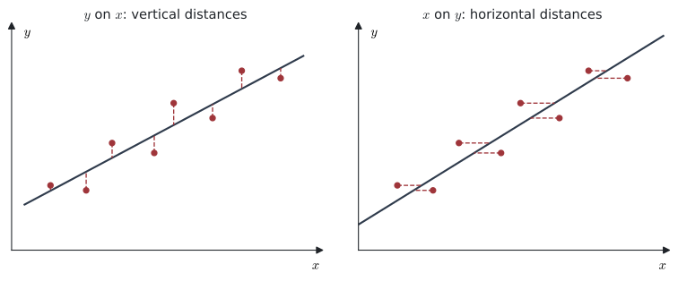
The two regression lines Not in the formula booklet

Regression line of \(y\) on \(x\): \(\quad y = ax + b\)

• \(x\) is the independent variable; \(y\) is the dependent variable.
• It minimises the sum of the squares of the vertical distances.
• Use it to estimate \(y\) from a given value of \(x\).

Regression line of \(x\) on \(y\): \(\quad x = cy + d\)

• \(y\) is the independent variable; \(x\) is the dependent variable.
• It minimises the sum of the squares of the horizontal distances.
• Use it to estimate \(x\) from a given value of \(y\).

• \(a\): the gradient of the \(y\) on \(x\) line
• \(b\): the \(y\)-intercept of the \(y\) on \(x\) line
• \(c\), \(d\): the constants in the \(x\) on \(y\) line

The syllabus says technology should be used to find the regression equations.

Both lines pass through the mean point

The regression line of \(y\) on \(x\) and the regression line of \(x\) on \(y\) both pass through \((\bar{x}, \bar{y})\). So the two lines intersect at the mean point. The two lines are the same line only when \(r = 1\) or \(r = -1\).

The IB writes the \(y\) on \(x\) line as \(y = ax + b\): \(a\) is the gradient and \(b\) is the \(y\)-intercept. (Be careful: some books and calculators use \(y = a + bx\), where the letters are the other way round.)

The regression line of \(y\) on \(x\)

Example 1 Find the regression line of \(y\) on \(x\) for the revision data of Section 17.1:

\(x\) (hours)	2	3	5	6	8	9	11	12	14	15
\(y\) (errors)	31	33	27	29	22	24	18	19	13	15

Interpret the values of \(a\) and \(b\) in this context.

Solution

GDC (Linear Regression (mx+b)): \(m = -1.4712\ldots\) and \(b = 35.605\ldots\), so

\[ y = -1.47x + 35.6 \quad \text{(3 s.f.)} \]

• \(a = -1.47\): for each extra hour of revision, the number of errors decreases by about \(1.47\), on average.
• \(b = 35.6\): a student who does no revision would be expected to make about \(36\) errors. (Be careful: \(x = 0\) is just outside the data, which runs from \(2\) to \(15\) hours.)

Paper 2 — regression lines on the TI-Nspire CX II

Enter the data in Lists & Spreadsheet (columns xx and yy).

\(y\) on \(x\): Menu → Statistics → Stat Calculations → Linear Regression (mx+b), with X List: xx, Y List: yy. The line is \(y = mx + b\), so the IB’s \(a\) is the calculator’s m.

\(x\) on \(y\): do the same, but swap the lists: X List: yy, Y List: xx. The output \(y = mx + b\) now means \(x = my + b\).

To draw the line, put the scatter diagram in Data & Statistics and choose Menu → Analyze → Regression → Show Linear (mx+b).

Interpreting \(a\) and \(b\)

Interpreting \(y = ax + b\) in context

• Gradient \(a\): when \(x\) increases by \(1\) unit, \(y\) changes by about \(a\) units, on average. (\(a > 0\): \(y\) increases. \(a < 0\): \(y\) decreases.)
• Intercept \(b\): the predicted value of \(y\) when \(x = 0\). This only makes sense if \(x = 0\) is a sensible value, close to the data.

Always use the context and the units in your answer. “The gradient is \(-1.47\)” is not an interpretation.

Example 2 For 30 flats in one city, the regression line of price (\(y\) thousand dollars) on floor area (\(x\) m²) is \(y = 4.2x + 85\). The floor areas are between \(50\) m² and \(140\) m².

(a) Interpret the value \(4.2\).

(b) Explain why the value \(85\) has no real meaning here.

Solution

(a) Each extra square metre of floor area increases the price by about $4200, on average.

(b) \(85\) is the predicted price of a flat with floor area \(0\) m². No flat has zero floor area, and \(x = 0\) is far outside the data (\(50\) to \(140\) m²). So \(b = 85\) only tells us where the line crosses the \(y\)-axis.

Independent and dependent variables

Which line should you use? It depends on which variable is independent — not on which letter is called \(x\).

On a scatter diagram the independent variable goes on the horizontal axis and the dependent variable on the vertical axis.

Independent variable	Given value	To find	Use the regression line of
\(x\)	\(x\)	\(y\)	\(y\) on \(x\)
\(y\)	\(y\)	\(x\)	\(x\) on \(y\)

In an experiment, the variable that is set by the experimenter (time, load, dose, temperature, …) is the independent variable. We usually assume it is measured accurately, and that the dependent variable has some random error. The least-squares line measures the errors in the dependent variable, so we regress the dependent variable on the independent one.

Example 3 In an experiment, a student hangs different loads (\(w\) newtons) on a spring and measures its length (\(L\) cm).

\(w\)	0.5	1.0	1.5	2.0	2.5	3.0	3.5	4.0
\(L\)	12.3	13.1	14.2	14.8	16.0	16.6	17.9	18.4

(a) Find the equation of a suitable regression line.

(b) Interpret the gradient and the intercept.

Solution

(a) The student chooses the loads, so \(w\) is the independent variable. We need the regression line of \(L\) on \(w\).

GDC (X List: \(w\), Y List: \(L\)): \(\;L = 1.79w + 11.4\) (3 s.f.), with \(r = 0.997\).

(b) Gradient: each extra newton of load stretches the spring by about \(1.79\) cm. Intercept: with no load, the spring is about \(11.4\) cm long (its natural length). Here \(w = 0\) is close to the data, so this value is sensible.

The regression line of \(x\) on \(y\)

SL 4.10

When both variables are random (neither is controlled), either line can be found. Use \(y\) on \(x\) to estimate \(y\), and \(x\) on \(y\) to estimate \(x\).

Do not rearrange the \(y\) on \(x\) line

The regression line of \(x\) on \(y\) is not found by making \(x\) the subject of \(y = ax + b\). The two lines minimise different distances, so they are different lines. Always use the GDC with the lists swapped.

Example 4 Eight pairs of observations are shown.

\(x\)	15	22	30	38	44	51	57	63
\(y\)	82	70	73	55	58	41	40	26

(a) Find the regression line of \(y\) on \(x\) and the regression line of \(x\) on \(y\).

(b) Find the point where the two lines intersect, and comment.

Solution

(a) GDC with X List \(x\), Y List \(y\): \(\quad y = -1.09x + 99.2\) (3 s.f.).

GDC with X List \(y\), Y List \(x\): \(\quad x = -0.860y + 87.8\) (3 s.f.).

(b) Solve the two equations together (use the unrounded values from the GDC, or the intersection tool on a Graphs page):

\[ x = 40.0, \qquad y = 55.6 \text{ (3 s.f.)} \]

The mean values are \(\bar{x} = \dfrac{320}{8} = 40\) and \(\bar{y} = \dfrac{445}{8} = 55.625\). So the two lines intersect at the mean point \((\bar{x}, \bar{y})\), as expected.

Figure 2: Both regression lines pass through the mean point

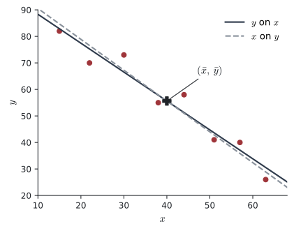
Here \(r = -0.968\), so the correlation is strong and the two lines are close together.

Because both lines pass through \((\bar{x}, \bar{y})\), you can find the mean point without a calculator by solving the two regression equations simultaneously. This is a common Paper 1 question.

Using your GDC

Task	TI-Nspire CX II (Lists & Spreadsheet)
\(y\) on \(x\)	Menu → Statistics → Stat Calculations → Linear Regression (mx+b), X List = \(x\), Y List = \(y\). Then \(a = m\), \(b = b\).
\(x\) on \(y\)	Same menu, but X List = \(y\), Y List = \(x\). The output means \(x = my + b\).
\(r\)	Shown on the same output screen.
Draw the line	Data & Statistics → Menu → Analyze → Regression → Show Linear (mx+b)

Give the coefficients to 3 significant figures, but keep the full values in the calculator for any further working.

Common errors

✗ Wrong	✓ Right	Why
Rearranging \(y = ax + b\) to get the \(x\) on \(y\) line	Use the GDC with the lists swapped	The two lines minimise different distances.
Always using “\(y\) on \(x\)” because the letters say so	Regress the dependent variable on the independent one	The context decides, not the letters.
Reading a from Linear Regression (a+bx) as the gradient	In \(y = a + bx\), the gradient is \(b\)	Use (mx+b) and match \(m\) with the IB’s \(a\).
“The gradient is \(-1.47\).”	“Each extra hour, about \(1.47\) fewer errors.”	An interpretation needs the context and the units.
Interpreting \(b\) when \(x = 0\) is impossible	Say that \(b\) has no practical meaning	\(x = 0\) may be far outside the data.
Rounding \(a\) and \(b\) early, then solving	Keep full GDC values	Rounded coefficients can move the answer.

Exercises

1 For each situation, state which regression line should be used.

(a) A teacher sets the length of a revision session (\(t\) minutes) and measures the students’ quiz scores (\(s\)). She wants to predict \(s\) for \(t = 45\).

(b) The heights (\(h\)) and masses (\(m\)) of 40 randomly chosen adults are measured. We want to estimate \(h\) for a person with \(m = 70\).

(c) For the same adults, we want to estimate \(m\) for a person with \(h = 175\).

Solution

(a) \(t\) is controlled (independent): the regression line of \(s\) on \(t\).

(b) Both are random. We want \(h\) from \(m\): the regression line of \(h\) on \(m\).

(c) We want \(m\) from \(h\): the regression line of \(m\) on \(h\).

2 Paper 1 The cost of a party (\(y\) dollars) for \(x\) guests is modelled by the regression line \(y = 12.5x + 180\), for \(20 \le x \le 80\). Interpret the values \(12.5\) and \(180\).

Solution

\(12.5\): each extra guest adds about $12.50 to the cost.

\(180\): the fixed cost (for example renting the room) that is paid whatever the number of guests. (Strictly, \(x = 0\) is outside the data, so this is an estimate.)

3 Paper 2 A shop records its weekly advertising spend (\(x\) hundred dollars) and its weekly sales (\(y\) thousand dollars).

\(x\)	1	2	3	4	5	6	7	8
\(y\)	12.1	13.8	15.2	15.9	18.3	19.0	20.7	22.4

(a) Find \(r\).

(b) Find the regression line of \(y\) on \(x\).

(c) Interpret the gradient.

Solution

(a) \(r = 0.996\) (3 s.f.).

(b) \(y = 1.43x + 10.7\) (3 s.f.).

(c) Each extra $100 spent on advertising goes with about $1430 more in weekly sales, on average.

4 Paper 2 For the data below, find

(a) the regression line of \(y\) on \(x\),

(b) the regression line of \(x\) on \(y\),

(c) the mean point.

\(x\)	4	7	9	12	15	18
\(y\)	30	26	27	20	18	13

Solution

(a) \(y = -1.21x + 35.4\) (3 s.f.).

(b) \(x = -0.792y + 28.5\) (3 s.f.).

(c) \(\bar{x} = \dfrac{65}{6} = 10.8\), \(\bar{y} = \dfrac{134}{6} = 22.3\) (3 s.f.). Both lines pass through \((10.8, 22.3)\).

5 Paper 1 For a set of data, the regression line of \(y\) on \(x\) is \(y = 0.5x + 4\) and the regression line of \(x\) on \(y\) is \(x = 1.5y - 3.5\). Find \(\bar{x}\) and \(\bar{y}\).

Solution

Both lines pass through \((\bar{x}, \bar{y})\). Substitute the first into the second:

\[ x = 1.5(0.5x + 4) - 3.5 = 0.75x + 2.5 \;\Longrightarrow\; 0.25x = 2.5 \;\Longrightarrow\; x = 10 . \]

Then \(y = 0.5 \times 10 + 4 = 9\). So \(\bar{x} = 10\), \(\bar{y} = 9\).

6 Paper 2 For the data below, find the regression line of \(y\) on \(x\) and rearrange it to make \(x\) the subject. Then find the regression line of \(x\) on \(y\) and compare.

\(x\)	1	3	4	6	8	9
\(y\)	4	5	8	7	10	12

Solution

\(y\) on \(x\): \(y = 0.925x + 2.89\). Rearranged: \(x = \dfrac{y - 2.89}{0.925} = 1.08y - 3.12\) (3 s.f.).

\(x\) on \(y\) (GDC, lists swapped): \(x = 0.956y - 2.16\) (3 s.f.).

The two equations are different. The rearranged \(y\) on \(x\) line is not the \(x\) on \(y\) regression line.

7 Paper 1 For 12 pairs of data, \(\sum x = 240\) and \(\sum y = 1056\). The regression line of \(y\) on \(x\) has gradient \(1.8\). Find its equation.

Solution

\(\bar{x} = \dfrac{240}{12} = 20\), \(\bar{y} = \dfrac{1056}{12} = 88\). The line passes through \((20, 88)\):

\[ 88 = 1.8 \times 20 + b \;\Longrightarrow\; b = 52 . \qquad y = 1.8x + 52 . \]

8 Paper 1 The boiling point of water (\(y\) °C) at altitude \(x\) km, for \(0 \le x \le 4\), is modelled by \(y = -3.3x + 100.1\). Interpret the gradient and the intercept.

Solution

Gradient: for each extra kilometre of altitude, the boiling point falls by about \(3.3\) °C.

Intercept: at sea level (\(x = 0\), inside the data) water boils at about \(100.1\) °C.

9 Paper 1 For adult men with heights \(160 \le x \le 195\) cm, the regression line of shoe size (\(y\)) on height is \(y = 0.18x - 22.6\).

(a) Interpret the value \(0.18\).

(b) Does the value \(-22.6\) have a meaning here? Explain.

Solution

(a) Each extra centimetre of height goes with a shoe size about \(0.18\) larger, on average (so about one shoe size for every \(5.6\) cm).

(b) No. It is the predicted shoe size for a height of \(0\) cm, which is impossible and far outside the data. A negative shoe size has no meaning.

10 Paper 2 In an experiment, a fixed amount of gas is heated to a chosen temperature (\(T\) °C), and its volume (\(V\) litres) is measured.

\(T\)	0	10	20	30	40	50
\(V\)	22.4	23.3	24.1	25.0	25.7	26.6

Find the equation of a suitable regression line, and interpret its gradient.

Solution

The temperature is chosen, so \(T\) is independent: use the regression line of \(V\) on \(T\).

GDC: \(V = 0.0831T + 22.4\) (3 s.f.).

The volume increases by about \(0.0831\) litres for each \(1\) °C rise in temperature.