18.1 Discrete Random Variables and Expected Value
SL 4.7
- what a random variable is, and the difference between discrete and continuous random variables
- how a probability distribution is given: as a table or as a formula
- that all the probabilities add up to \(1\), and how to use this to find unknowns
- how to find the expected value (mean) \(\mathrm{E}(X)\) and the mode
- what a fair game is, and how to use \(\mathrm{E}(X)\) in applications
Random variables
A random variable gives a number to each outcome of a random experiment. We write random variables with capital letters, such as \(X\), and the values they take with small letters, such as \(x\).
A discrete random variable can take only separate, exact values, such as \(x = 0, 1, 2, 3, \ldots\) There may be a finite number of values, or an infinite list of them. A discrete random variable usually comes from counting.
- the number of buses that arrive late at a stop in one morning
- the number of goals scored in a football match
- the number of times you must spin a spinner until it lands on red
A continuous random variable can take any value in an interval. It usually comes from measuring. For example, the time \(T\) minutes that a student needs to finish a test could be any value with \(20 < t < 60\). Continuous random variables are studied in Unit 19.
Discrete or continuous? Not in the formula booklet
- Discrete: you count it. The values are separate (often whole numbers).
- Continuous: you measure it. Any value in an interval is possible.
Probability distributions
Each value \(x_1, x_2, \ldots, x_n\) of a discrete random variable \(X\) has a probability \(\mathrm{P}(X = x_1), \mathrm{P}(X = x_2), \ldots\) The list of values together with their probabilities is the probability distribution of \(X\).
Conditions for a probability distribution Not in the formula booklet
\[ 0 \le \mathrm{P}(X = x) \le 1 \quad \text{for every } x \qquad\text{and}\qquad \sum_{\text{all } x} \mathrm{P}(X = x) = 1 \]
- \(X\): a discrete random variable
- \(x\): a value that \(X\) can take
- \(\mathrm{P}(X = x)\): the probability that \(X\) takes the value \(x\)
A probability distribution is usually given in one of two ways.
As a table:
| \(x\) | \(1\) | \(2\) | \(3\) | \(4\) |
|---|---|---|---|---|
| \(\mathrm{P}(X = x)\) | \(0.1\) | \(0.3\) | \(0.4\) | \(0.2\) |
As a formula, for example \(\mathrm{P}(X = x) = \dfrac{x}{10}\) for \(x = 1, 2, 3, 4\).
The table is easy to read. The formula is short, but you usually substitute each value of \(x\) and make a table anyway.
Example 1 (a) Show that \(\mathrm{P}(X = x) = \dfrac{x^2 + 2}{38}\), \(\;x = 1, 2, 3, 4\), is a probability distribution.
(b) Show that \(\mathrm{P}(Y = y) = \dbinom{4}{y}(0.3)^y(0.7)^{4 - y}\), \(\;y = 0, 1, 2, 3, 4\), is a probability distribution.
(c) The random variable \(W\) has \(\mathrm{P}(W = w) = k(w + 2)\) for \(w = 0, 1, 2, 3\). Find the value of \(k\).
(a) Substitute each value:
| \(x\) | \(1\) | \(2\) | \(3\) | \(4\) |
|---|---|---|---|---|
| \(\mathrm{P}(X = x)\) | \(\frac{3}{38}\) | \(\frac{6}{38}\) | \(\frac{11}{38}\) | \(\frac{18}{38}\) |
All the probabilities are between \(0\) and \(1\), and \(\dfrac{3 + 6 + 11 + 18}{38} = \dfrac{38}{38} = 1\). So it is a probability distribution.
(b)
| \(y\) | \(0\) | \(1\) | \(2\) | \(3\) | \(4\) |
|---|---|---|---|---|---|
| \(\mathrm{P}(Y = y)\) | \(0.2401\) | \(0.4116\) | \(0.2646\) | \(0.0756\) | \(0.0081\) |
Each value is between \(0\) and \(1\), and the sum is \(0.2401 + 0.4116 + 0.2646 + 0.0756 + 0.0081 = 1\).
(A quicker way: by the binomial theorem, the five terms are the expansion of \((0.3 + 0.7)^4 = 1^4 = 1\). See Section 4.1.)
(c) The probabilities must add up to \(1\):
\[ k(2) + k(3) + k(4) + k(5) = 14k = 1 \;\Longrightarrow\; k = \frac{1}{14} . \]
To find a distribution from a situation, list every possible value of \(X\) first, then find each probability (a tree diagram often helps). Finally, check that the total is \(1\).
Example 2 A bag contains 5 green and 3 yellow counters. Two counters are taken at random, without replacement. \(X\) is the number of green counters taken.
(a) Find the probability distribution of \(X\) in a table.
(b) Hence find \(\mathrm{P}(X = 1 \mid X \le 1)\).
(a) \(X\) can be \(0\), \(1\) or \(2\).
\[ \begin{aligned} \mathrm{P}(X = 0) &= \frac{3}{8} \times \frac{2}{7} = \frac{6}{56}, \\ \mathrm{P}(X = 1) &= \frac{5}{8} \times \frac{3}{7} + \frac{3}{8} \times \frac{5}{7} = \frac{30}{56}, \\ \mathrm{P}(X = 2) &= \frac{5}{8} \times \frac{4}{7} = \frac{20}{56} \end{aligned} \]
| \(x\) | \(0\) | \(1\) | \(2\) |
|---|---|---|---|
| \(\mathrm{P}(X = x)\) | \(\frac{3}{28}\) | \(\frac{15}{28}\) | \(\frac{5}{14}\) |
Check: \(\dfrac{6 + 30 + 20}{56} = 1\).
(b) This is a conditional probability (see Unit 16):
\[ \mathrm{P}(X = 1 \mid X \le 1) = \frac{\mathrm{P}(X = 1)}{\mathrm{P}(X \le 1)} = \frac{\frac{15}{28}}{\frac{3}{28} + \frac{15}{28}} = \frac{15}{18} = \frac{5}{6} . \]
Example 3 A fair six-sided dice has faces labelled \(1, 2, 2, 4, 4, 4\). It is thrown twice, and \(X\) is the total of the two scores.
(a) Write down the possible values of \(X\). \(\quad\)
(b) Find the probability distribution of \(X\). \(\quad\)
(c) Find \(\mathrm{P}(X \ge 5 \mid X \le 6)\).
(a) On one throw, \(\mathrm{P}(1) = \frac{1}{6}\), \(\mathrm{P}(2) = \frac{2}{6}\), \(\mathrm{P}(4) = \frac{3}{6}\). The possible totals are \(2, 3, 4, 5, 6, 8\). (A total of \(7\) is impossible.)
(b) A sample-space table gives the totals of the \(6 \times 6 = 36\) equally likely pairs:
| \(+\) | \(1\) | \(2\) | \(2\) | \(4\) | \(4\) | \(4\) |
|---|---|---|---|---|---|---|
| \(1\) | 2 | 3 | 3 | 5 | 5 | 5 |
| \(2\) | 3 | 4 | 4 | 6 | 6 | 6 |
| \(2\) | 3 | 4 | 4 | 6 | 6 | 6 |
| \(4\) | 5 | 6 | 6 | 8 | 8 | 8 |
| \(4\) | 5 | 6 | 6 | 8 | 8 | 8 |
| \(4\) | 5 | 6 | 6 | 8 | 8 | 8 |
| \(x\) | \(2\) | \(3\) | \(4\) | \(5\) | \(6\) | \(8\) |
|---|---|---|---|---|---|---|
| \(\mathrm{P}(X = x)\) | \(\frac{1}{36}\) | \(\frac{4}{36}\) | \(\frac{4}{36}\) | \(\frac{6}{36}\) | \(\frac{12}{36}\) | \(\frac{9}{36}\) |
Check: \(1 + 4 + 4 + 6 + 12 + 9 = 36\) ✓. The distribution is shown in Figure 1.
(c)
\[ \mathrm{P}(X \ge 5 \mid X \le 6) = \frac{\mathrm{P}(5 \le X \le 6)}{\mathrm{P}(X \le 6)} = \frac{6 + 12}{1 + 4 + 4 + 6 + 12} = \frac{18}{27} = \frac{2}{3} . \]
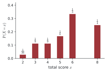
A bar chart like Figure 1 is a good picture of a discrete distribution: one bar for each value, with height equal to its probability.
Expected value (mean)
Suppose an experiment is repeated a very large number of times. The expected value \(\mathrm{E}(X)\) is the long-run average value of \(X\). It is found by weighting each value by its probability.
Expected value of a discrete random variable In the formula booklet
\[ \mathrm{E}(X) = \sum_{i=1}^{k} x_i\,\mathrm{P}(X = x_i) \]
In short: \(\mathrm{E}(X) = \sum x\,\mathrm{P}(X = x)\), a sum over all values \(x\) of \(X\).
- \(\mathrm{E}(X)\): the expected value (mean) of \(X\)
- \(x_i\): the possible values of \(X\) (\(x_1, x_2, \ldots, x_k\))
- \(\mathrm{P}(X = x_i)\): the probability that \(X\) takes the value \(x_i\)
- \(k\): the number of possible values of \(X\)
\(\mathrm{E}(X)\) is also called the mean of \(X\), and is often written \(\mu\). Compare it with the mean of a frequency table, \(\bar{x} = \dfrac{\sum f x}{\sum f}\): the relative frequencies \(\dfrac{f}{\sum f}\) are replaced by probabilities.
The same idea works for any function of \(X\). For example
\[ \mathrm{E}(X^2) = \sum x^2\,\mathrm{P}(X = x), \qquad \text{and in general} \qquad \mathrm{E}\big(g(X)\big) = \sum g(x)\,\mathrm{P}(X = x) . \]
The mode of \(X\) is the value with the largest probability. In general the mean and the mode are different, and \(\mathrm{E}(X)\) does not have to be a possible value of \(X\).
Example 4 A regular five-sided spinner is labelled \(1, 2, 2, 2, 5\). A player spins it once and wins the amount \(W\) shown below.
| Number on spinner | \(1\) | \(2\) | \(5\) |
|---|---|---|---|
| Winnings \(W\) | $0 | $1 | $8 |
(a) Find the probability distribution of \(W\).
(b) Find \(\mathrm{E}(W)\) and the mode of \(W\). \(\quad\) (c) It costs $2.50 to play. Find the player’s expected gain per game.
(a)
| \(w\) | \(0\) | \(1\) | \(8\) |
|---|---|---|---|
| \(\mathrm{P}(W = w)\) | \(\frac{1}{5}\) | \(\frac{3}{5}\) | \(\frac{1}{5}\) |
(b) \(\mathrm{E}(W) = 0 \times \dfrac{1}{5} + 1 \times \dfrac{3}{5} + 8 \times \dfrac{1}{5} = \dfrac{11}{5} = \$2.20\).
The mode is \(W = \$1\) (largest probability, \(\frac{3}{5}\)). Notice that the mean and the mode are different.
(c) Expected gain \(= 2.20 - 2.50 = -\$0.30\). On average the player loses 30 cents per game.
Fair games
Let \(X\) be the gain (profit) of a player in one game. A negative value means a loss.
Fair game Not in the formula booklet
A game is fair if the expected gain of the player is zero: \(\;\mathrm{E}(X) = 0\).
- \(X\): the gain of the player in one game (a loss is a negative gain)
- \(\mathrm{E}(X)\): the expected gain of the player
If \(\mathrm{E}(X) < 0\), the game favours the organiser (a casino or a stall at a fair, for example). If \(\mathrm{E}(X) > 0\), it favours the player.
Example 5 Ana tosses two fair coins and Ben tosses one fair coin. They compare their numbers of heads.
- If Ana gets more heads, Ben pays Ana $2.
- If Ben gets more heads, Ana pays Ben $6.
- If they get the same number of heads, Ana pays Ben $1.
(a) Find Ana’s expected gain. Is the game fair? \(\qquad\)
(b) Ben wants the game to be fair. How much should he pay Ana when she gets more heads?
(a) Let \(A\) = Ana’s heads and \(B\) = Ben’s heads. \(\mathrm{P}(A = 0) = \frac{1}{4}\), \(\mathrm{P}(A = 1) = \frac{1}{2}\), \(\mathrm{P}(A = 2) = \frac{1}{4}\); \(\;\mathrm{P}(B = 0) = \mathrm{P}(B = 1) = \frac{1}{2}\).
\[ \begin{aligned} \mathrm{P}(A > B) &= \mathrm{P}(1, 0) + \mathrm{P}(2, 0) + \mathrm{P}(2, 1) = \tfrac{1}{4} + \tfrac{1}{8} + \tfrac{1}{8} = \tfrac{1}{2} \\ \mathrm{P}(A = B) &= \mathrm{P}(0, 0) + \mathrm{P}(1, 1) = \tfrac{1}{8} + \tfrac{1}{4} = \tfrac{3}{8} \\ \mathrm{P}(A < B) &= \mathrm{P}(0, 1) = \tfrac{1}{8} \end{aligned} \]
Let \(G\) be Ana’s gain in dollars.
| \(g\) | \(2\) | \(-1\) | \(-6\) |
|---|---|---|---|
| \(\mathrm{P}(G = g)\) | \(\frac{1}{2}\) | \(\frac{3}{8}\) | \(\frac{1}{8}\) |
\[ \mathrm{E}(G) = 2 \times \frac{1}{2} - 1 \times \frac{3}{8} - 6 \times \frac{1}{8} = 1 - \frac{9}{8} = -\frac{1}{8} . \]
Ana expects to lose \(12.5\) cents per game, so the game is not fair (it favours Ben).
(b) Let Ben pay $\(m\). Then \(\;\dfrac{1}{2}m - \dfrac{3}{8} - \dfrac{6}{8} = 0\), so \(m = \dfrac{9}{4} = \$2.25\).
Applications
Expected value is used by businesses, insurance companies and game designers to make decisions. When the amounts depend on an unknown (such as a fee), write the gain in terms of the unknown and form an equation.
Example 6 To play a game, a player pays an entrance fee of $\(m\). Two fair six-sided dice are then rolled.
- If both dice show a six, the player receives \(6m\).
- If exactly one dice shows a six, the player receives \(2m\).
- Otherwise the player receives nothing.
(a) Complete the table for the player’s profit.
(b) Show that the expected profit is \(-\dfrac{5m}{18}\).
(c) The expected loss per game is 45 cents. Find the entrance fee.
| Profit ($) | \(-m\) | \(m\) | \(5m\) |
|---|---|---|---|
| Probability |
(a) Profit = amount received \(-\) fee. Two sixes: \(6m - m = 5m\). One six: \(2m - m = m\). No six: \(-m\).
\(\mathrm{P}(\text{two sixes}) = \frac{1}{36}\), \(\;\mathrm{P}(\text{exactly one six}) = 2 \times \frac{1}{6} \times \frac{5}{6} = \frac{10}{36}\), \(\;\mathrm{P}(\text{no six}) = \frac{25}{36}\).
| Profit ($) | \(-m\) | \(m\) | \(5m\) |
|---|---|---|---|
| Probability | \(\frac{25}{36}\) | \(\frac{10}{36}\) | \(\frac{1}{36}\) |
(b)
\[ \mathrm{E}(\text{profit}) = -m \times \frac{25}{36} + m \times \frac{10}{36} + 5m \times \frac{1}{36} = \frac{-25m + 10m + 5m}{36} = -\frac{10m}{36} = -\frac{5m}{18} . \]
(c) \(\dfrac{5m}{18} = 0.45 \;\Longrightarrow\; m = \dfrac{0.45 \times 18}{5} = 1.62\). The fee is $1.62.
Common errors
| ✗ Wrong | ✓ Right | Why |
|---|---|---|
| Forgetting a value of \(X\) (for example \(X = 0\)) | List all values first | Then check that the probabilities add up to \(1\). |
| \(\mathrm{E}(X) = \dfrac{\sum x}{n}\) | \(\mathrm{E}(X) = \sum x\,\mathrm{P}(X = x)\) | Each value must be weighted by its probability. |
| “\(\mathrm{E}(X)\) must be a possible value of \(X\)” | \(\mathrm{E}(X) = 2.2\) is fine | It is a long-run average, not an outcome. |
| Using the winnings, not the profit, to judge fairness | Profit = winnings \(-\) cost | A fair game has expected gain \(0\). |
| \(\mathrm{P}(X = 1 \mid X \le 1) = \mathrm{P}(X = 1)\) | Divide by \(\mathrm{P}(X \le 1)\) | “Given that” reduces the sample space. |
Exercises
1 State whether each random variable is discrete or continuous.
(a) The number of emails received in one hour.
(b) The time taken to run 100 m. (c) The number of goals in a hockey match.
(d) The mass of an apple.
(a) Discrete (a count).
(b) Continuous (a measurement).
(c) Discrete.
(d) Continuous.
2 The random variable \(X\) has \(\mathrm{P}(X = x) = kx^2\) for \(x = 1, 2, 3\). Find \(k\) and \(\mathrm{P}(X \ge 2)\).
\(k(1 + 4 + 9) = 14k = 1\), so \(k = \dfrac{1}{14}\). \(\quad \mathrm{P}(X \ge 2) = \dfrac{4 + 9}{14} = \dfrac{13}{14}\).
3 The probability distribution of \(X\) is shown. Find \(a\) and \(\mathrm{E}(X)\).
| \(x\) | \(1\) | \(2\) | \(3\) | \(4\) |
|---|---|---|---|---|
| \(\mathrm{P}(X = x)\) | \(0.2\) | \(a\) | \(0.35\) | \(2a\) |
\(0.2 + a + 0.35 + 2a = 1 \Rightarrow 3a = 0.45 \Rightarrow a = 0.15\).
\(\mathrm{E}(X) = 1(0.2) + 2(0.15) + 3(0.35) + 4(0.3) = 0.2 + 0.3 + 1.05 + 1.2 = 2.75\).
4 \(\mathrm{P}(X = x) = \dfrac{x + 1}{k}\) for \(x = 0, 1, 2, 3, 4\). Find \(k\), \(\mathrm{E}(X)\) and the mode of \(X\).
\(\dfrac{1 + 2 + 3 + 4 + 5}{k} = 1\), so \(k = 15\).
\(\mathrm{E}(X) = \dfrac{0 \times 1 + 1 \times 2 + 2 \times 3 + 3 \times 4 + 4 \times 5}{15} = \dfrac{40}{15} = \dfrac{8}{3}\).
The mode is \(4\) (largest probability, \(\frac{5}{15}\)).
5 Two cards are taken at random, without replacement, from four cards numbered \(1, 2, 3, 4\). \(X\) is the larger of the two numbers. Find the distribution of \(X\) and \(\mathrm{E}(X)\).
There are \(\binom{4}{2} = 6\) equally likely pairs: \(\{1,2\}, \{1,3\}, \{1,4\}, \{2,3\}, \{2,4\}, \{3,4\}\).
| \(x\) | \(2\) | \(3\) | \(4\) |
|---|---|---|---|
| \(\mathrm{P}(X = x)\) | \(\frac{1}{6}\) | \(\frac{2}{6}\) | \(\frac{3}{6}\) |
\(\mathrm{E}(X) = \dfrac{2 + 6 + 12}{6} = \dfrac{20}{6} = \dfrac{10}{3}\).
6 The distribution of \(X\) is shown, and \(\mathrm{E}(X) = 1.6\). Find \(p\) and \(q\).
| \(x\) | \(0\) | \(1\) | \(2\) | \(3\) |
|---|---|---|---|---|
| \(\mathrm{P}(X = x)\) | \(0.1\) | \(p\) | \(q\) | \(0.2\) |
Sum: \(0.1 + p + q + 0.2 = 1\), so \(p + q = 0.7\).
Mean: \(p + 2q + 0.6 = 1.6\), so \(p + 2q = 1\).
Subtracting: \(q = 0.3\), then \(p = 0.4\).
7 A game costs $3 to play. A fair dice is rolled once. A six wins $10, a four or a five wins $3, and anything else wins nothing.
(a) Find the expected profit per game.
(b) What prize for a six would make the game fair?
(a) Profit: six \(\to 7\) (prob \(\frac{1}{6}\)); four or five \(\to 0\) (prob \(\frac{2}{6}\)); otherwise \(\to -3\) (prob \(\frac{3}{6}\)).
\(\mathrm{E} = \dfrac{7}{6} + 0 - \dfrac{9}{6} = -\dfrac{1}{3}\). The player expects to lose about 33 cents per game.
(b) Prize $\(x\) for a six: \(\dfrac{x - 3}{6} - \dfrac{9}{6} = 0 \Rightarrow x - 3 = 9 \Rightarrow x = 12\). The prize should be $12.
8 A bag contains 4 red and 6 white balls. One ball is taken at random. A red ball wins $\(k\); a white ball loses $2. Find \(k\) so that the game is fair.
\(\mathrm{E}(\text{gain}) = 0.4k - 0.6 \times 2 = 0 \Rightarrow 0.4k = 1.2 \Rightarrow k = 3\).
9 For the distribution below, find \(\mathrm{E}(X)\), \(\mathrm{E}(X^2)\) and \(\mathrm{E}\!\left(\dfrac{1}{X}\right)\).
| \(x\) | \(1\) | \(2\) | \(4\) |
|---|---|---|---|
| \(\mathrm{P}(X = x)\) | \(0.5\) | \(0.3\) | \(0.2\) |
\(\mathrm{E}(X) = 0.5 + 0.6 + 0.8 = 1.9\).
\(\mathrm{E}(X^2) = 1(0.5) + 4(0.3) + 16(0.2) = 0.5 + 1.2 + 3.2 = 4.9\).
\(\mathrm{E}\!\left(\dfrac{1}{X}\right) = 1(0.5) + \dfrac{1}{2}(0.3) + \dfrac{1}{4}(0.2) = 0.5 + 0.15 + 0.05 = 0.7\).
(Notice that \(\mathrm{E}(X^2) \ne [\mathrm{E}(X)]^2 = 3.61\).)
10 An insurance company sells a one-year phone policy for $\(P\). In a year, the probability of a claim of $600 is \(0.03\), and the probability of a claim of $200 is \(0.1\). Otherwise there is no claim. Find \(P\) so that the company’s expected profit per policy is $12.
Expected payout \(= 600(0.03) + 200(0.1) = 18 + 20 = \$38\).
Expected profit \(= P - 38 = 12\), so \(P = \$50\).