9.6 Key Features of Graphs
SL 2.3 SL 2.4
- what the graph of a function \(y = f(x)\) is, and how to test whether a point lies on it
- the difference between the command terms draw and sketch, and what to label
- the key features of a graph: intercepts, zeros, maximum and minimum points, vertex, symmetry and asymptotes
- how to sketch a graph from an equation, from given information, or from a real-life context
- how to use a GDC to graph functions (including sums and differences of functions) and find key features
- how to transfer a graph from the calculator screen to paper
The graph of a function
The graph of a function \(f\) is the set of all points \((x, y)\) with \(y = f(x)\). We call \(y = f(x)\) the equation of the graph.
A point on a graph Not in the formula booklet
The point \((a, b)\) lies on the graph of \(y = f(x)\) exactly when \(f(a) = b\).
So to test a point, substitute its \(x\)-coordinate into \(f\) and compare the result with its \(y\)-coordinate. If a point on the graph is given, this gives you an equation, which you can use to find an unknown constant.
“Draw” and “sketch”
IB questions use command terms. Two of them ask for a graph, but they ask for different things.
| Command term | What you must do |
|---|---|
| Draw | An accurate graph, usually on graph paper and to scale. Plot points correctly and join them with a smooth curve (use a ruler for straight lines). |
| Sketch | A graph that shows the general shape and the relevant features. It does not need to be to scale, but it must be labelled. |
In both cases the labels matter. Many marks are lost for a correct shape with no labels.
What to label on a graph
- both axes (\(x\) and \(y\), or the variables in the context, such as \(t\) and \(h\))
- the intercepts with both axes
- maximum and minimum points (the vertex of a parabola)
- asymptotes, as dashed lines with their equations
- the end points, if a domain is given
- the equation of each curve, if there is more than one
Key features of a graph
| Feature | Meaning | How to find it by hand |
|---|---|---|
| \(y\)-intercept | where the graph meets the \(y\)-axis | find \(f(0)\) |
| \(x\)-intercepts (zeros) | where the graph meets the \(x\)-axis | solve \(f(x) = 0\); the solutions are the roots of the equation |
| maximum / minimum | the highest / lowest point (locally or overall) | quadratics: the vertex (8.2); in general, calculus (Unit 25) or a GDC |
| line of symmetry | a line the graph is a mirror image in | quadratics: \(x = -\dfrac{b}{2a}\) (8.2) |
| vertical asymptote | a line \(x = k\) that the graph approaches but never meets | for a fraction, where the denominator is \(0\) (10.1) |
| horizontal asymptote | a line \(y = k\) that the graph approaches as \(x \to \pm\infty\) | what \(f(x)\) approaches for very large \(|x|\) (10.1) |
The words zero (of a function) and root (of an equation) mean the same \(x\)-values: the zeros of \(f\) are the roots of \(f(x) = 0\).
The methods for each family of functions are taught with that family: the vertex and axis of symmetry of a quadratic in Section 8.2, and the asymptotes of a rational function in Section 10.1. This section is about using the features: to sketch a graph from information or from a context, and to find them with technology.
Sketching from information
Sometimes you are not given an equation, only a list of facts. Then you build the sketch from the facts, one at a time. Many different curves may be correct: any curve that shows every fact is fine.
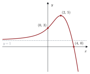
Example 1 Sketch a possible graph of a function \(f\), defined for all \(x \in \mathbb{R}\), with these properties:
- the \(y\)-intercept is \(3\);
- the only zero is \(x = 4\);
- there is a maximum point at \((2, 5)\), and no other maximum or minimum points;
- the line \(y = 1\) is a horizontal asymptote as \(x \to -\infty\);
- \(f(x) \to -\infty\) as \(x \to \infty\).
Plot the three points \((0, 3)\), \((2, 5)\) and \((4, 0)\), and draw \(y = 1\) as a dashed line.
On the left, the curve starts just above \(y = 1\) and rises (it cannot cross the \(x\)-axis, because the only zero is \(x = 4\)). It passes through \((0, 3)\), turns at \((2, 5)\), then falls through \((4, 0)\) and keeps falling.
Using technology to graph functions
On Paper 2 you can use a GDC. It is very good at finding key features that are hard by hand, for example the zeros of a cubic or the turning points of any curve. You can also graph sums and differences of functions directly: if \(f_1\) and \(f_2\) are defined, enter \(f_3(x) = f_1(x) + f_2(x)\) or \(f_3(x) = f_1(x) - f_2(x)\).
- Open a Graphs page and enter the function as \(f_1(x)\).
- Choose a good window: Menu → Window / Zoom → Window Settings (or Zoom – Fit).
- Zeros: Menu → Analyze Graph → Zero. Click to the left of the zero (lower bound), then to the right of it (upper bound).
- Minimum / maximum: Menu → Analyze Graph → Minimum (or Maximum), with lower and upper bounds in the same way.
- \(y\)-intercept: Menu → Trace → Graph Trace, then type
0and press enter. - Asymptotes: the GDC does not label them. Press ctrl + T for a split-screen table (or trace to large \(|x|\)) and see which value \(f(x)\) approaches.
Repeat steps 3–4 for each zero or turning point. Give answers to 3 significant figures unless the question says otherwise. To find where two graphs meet (Analyze Graph → Intersection), see Section 9.7.
Transferring a graph from screen to paper
When you copy a GDC graph into your answer:
- use the same domain as the question (the end points of the curve should be at the right \(x\)-values);
- mark the scale on the axes, or label the important points with their coordinates;
- keep the shape correct: turning points, intercepts and asymptotes in the right places, and the right behaviour at the ends;
- label everything the calculator showed you.
Example 2 Let \(f(x) = x^3 - 4x + 1\), for \(-2.5 \le x \le 2.5\).
(a) Use your GDC to find the zeros of \(f\).
(b) Find the coordinates of the local maximum and local minimum points.
(c) Find the coordinates of the end points, and hence sketch the graph.
(a) Using Analyze Graph → Zero three times: \(x = -2.11\), \(x = 0.254\), \(x = 1.86\).
(b) Local maximum \((-1.15,\, 4.08)\); local minimum \((1.15,\, -2.08)\).
(c) \(f(-2.5) = -15.625 + 10 + 1 = -4.625\) and \(f(2.5) = 15.625 - 10 + 1 = 6.625\). The end points are \((-2.5,\, -4.625)\) and \((2.5,\, 6.625)\).
The sketch starts at \((-2.5, -4.625)\), rises through \((-2.11, 0)\) to the maximum \((-1.15, 4.08)\), falls through the \(y\)-intercept \((0, 1)\) and \((0.254, 0)\) to the minimum \((1.15, -2.08)\), then rises through \((1.86, 0)\) to \((2.5, 6.625)\). Label all of these points on your sketch.
Sketching from a context
In a real-life context, the variables usually have names and units, and the domain is limited by the situation (for example, time cannot be negative). Label the axes with the variables and units.
Example 3 A ball is thrown upwards from a platform. Its height above the ground, in metres, \(t\) seconds after it is thrown is
\[ h(t) = 1.5 + 14t - 4.9t^2 . \]
(a) Write down the height from which the ball is thrown.
(b) Find the maximum height of the ball, and the time when this happens.
(c) Find the time when the ball hits the ground.
(d) Sketch the graph of \(h\) for the time the ball is in the air.
(a) \(h(0) = 1.5\) m.
(b) The vertex is at \(t = -\dfrac{14}{2 \times (-4.9)} = \dfrac{14}{9.8} = 1.43\) s (3 s.f.).
\(h\!\left(\dfrac{14}{9.8}\right) = 1.5 + \dfrac{14^2}{2 \times 9.8} = 1.5 + 10 = 11.5\) m.
(c) Solve \(1.5 + 14t - 4.9t^2 = 0\). On the GDC (Analyze Graph → Zero), or with the quadratic formula, \(t = 2.96\) s. The other root, \(t = -0.103\), is rejected because \(t \ge 0\).
(d) The domain is \(0 \le t \le 2.96\). The graph is part of a parabola, opening downwards. Label the axes \(t\) (s) and \(h\) (m), the start point \((0, 1.5)\), the maximum \((1.43, 11.5)\) and the end point \((2.96, 0)\).
Common errors
| ✗ Wrong | ✓ Right | Why |
|---|---|---|
| A correct curve with no labels | Label the axes, intercepts, turning points and asymptotes | “Sketch” still asks for the relevant features to be labelled. |
| Drawing an asymptote as a solid line, or leaving out its equation | A dashed line with its equation, e.g. \(x = 1\) | A solid line looks like part of the graph. |
| A curve that touches or crosses a vertical asymptote | The curve gets closer and closer but never meets it | At \(x = k\) the function is not defined. |
| Copying the GDC screen with the wrong domain | Use exactly the domain in the question | The end points are key features too. |
| Writing GDC answers like \(1.4841\) or \(1.5\) | \(1.48\) | Give 3 significant figures unless told otherwise. |
Exercises
1 The point \((2, 5)\) lies on the graph of \(y = x^3 - 2x + k\). Find \(k\). Does the point \((-1, 2)\) lie on the same graph?
\(8 - 4 + k = 5\), so \(k = 1\). The equation is \(y = x^3 - 2x + 1\).
At \(x = -1\): \(\;y = -1 + 2 + 1 = 2\). So yes, \((-1, 2)\) lies on the graph.
2 For \(y = x^2 - 6x + 5\), find the intercepts with both axes, the axis of symmetry and the vertex. Sketch the graph.
\(y\)-intercept: \((0, 5)\). \(\;x^2 - 6x + 5 = (x - 1)(x - 5) = 0\), so the \(x\)-intercepts are \((1, 0)\) and \((5, 0)\).
Axis of symmetry: \(x = -\dfrac{-6}{2} = 3\). Vertex: \(y = 9 - 18 + 5 = -4\), so \((3, -4)\), a minimum.
The sketch is a parabola opening upwards through these four points, with the dashed line \(x = 3\).
3 For \(y = \dfrac{x + 4}{x - 2}\), write down the equations of the asymptotes and find the intercepts with the axes.
Vertical asymptote \(x = 2\); horizontal asymptote \(y = \dfrac{1}{1} = 1\).
\(y\)-intercept: \(\dfrac{4}{-2} = -2\), so \((0, -2)\). \(\;x\)-intercept: \(x + 4 = 0\), so \((-4, 0)\).
4 Let \(f(x) = 3 - \dfrac{6}{x + 1}\), \(x \neq -1\).
(a) Write down the equations of the asymptotes.
(b) Find the intercepts.
(c) Sketch the graph.
(a) \(x = -1\) and \(y = 3\) (the fraction \(\dfrac{6}{x + 1} \to 0\) for large \(|x|\)).
(b) \(f(0) = 3 - 6 = -3\), so \((0, -3)\). \(\;3 - \dfrac{6}{x + 1} = 0 \Rightarrow x + 1 = 2 \Rightarrow x = 1\), so \((1, 0)\).
(c) Two branches: the right-hand branch passes through \((0, -3)\) and \((1, 0)\) and approaches \(y = 3\) from below; the left-hand branch lies above \(y = 3\) in the region \(x < -1\).
5 Let \(f(x) = x^4 - 5x^2 + 4\).
(a) Find the zeros of \(f\) and the \(y\)-intercept.
(b) Explain why the graph is symmetric in the \(y\)-axis.
(c) By writing \(f(x) = \left(x^2 - \frac{5}{2}\right)^2 - \frac{9}{4}\), find the minimum value of \(f\).
(a) \(x^4 - 5x^2 + 4 = (x^2 - 1)(x^2 - 4) = 0\), so \(x = \pm 1\) and \(x = \pm 2\). The \(y\)-intercept is \((0, 4)\).
(b) Only even powers of \(x\) appear, so \(f(-x) = f(x)\). The point \((-x, y)\) is on the graph whenever \((x, y)\) is.
(c) \(\left(x^2 - \frac{5}{2}\right)^2 \ge 0\), so the minimum value is \(-\dfrac{9}{4}\), when \(x^2 = \dfrac{5}{2}\), that is \(x = \pm\sqrt{\dfrac{5}{2}}\).
6 Question A says “Draw the graph of \(y = 2x - 1\) for \(0 \le x \le 4\) on the grid.” Question B says “Sketch the graph of \(y = 2x - 1\).” Explain what is different in your two answers.
For A you must be accurate: use the scale on the grid, plot points such as \((0, -1)\) and \((4, 7)\) correctly, join them with a ruler, and stop at the end points \(x = 0\) and \(x = 4\).
For B the graph only needs the correct general shape (a straight line with positive gradient) and the labelled key features: the intercepts \((0, -1)\) and \(\left(\frac{1}{2}, 0\right)\). It does not need to be to scale.
7 Let \(f(x) = x^3 - 2x^2 - 5x + 3\). Use your GDC to find the zeros of \(f\) and the coordinates of the local maximum and minimum points.
Zeros: \(x = -1.77\), \(x = 0.520\), \(x = 3.25\).
Local maximum \((-0.786,\, 5.21)\); local minimum \((2.12,\, -7.06)\).
8 Let \(f(x) = \dfrac{6}{1 + 2\mathrm{e}^{-x}}\).
(a) Find the \(y\)-intercept.
(b) Use your GDC to sketch the graph, and write down the equations of the two horizontal asymptotes.
(a) \(f(0) = \dfrac{6}{1 + 2} = 2\), so \((0, 2)\).
(b) As \(x \to \infty\), \(\mathrm{e}^{-x} \to 0\), so \(f(x) \to 6\). As \(x \to -\infty\), \(\mathrm{e}^{-x} \to \infty\), so \(f(x) \to 0\). The asymptotes are \(y = 0\) and \(y = 6\). The graph is an increasing “S” shape between them, through \((0, 2)\).
9 Let \(f(x) = x^2\) and \(g(x) = \dfrac{4}{x}\), for \(x > 0\).
(a) On your GDC, graph \(y = f(x) + g(x)\) for \(x > 0\).
(b) Find the coordinates of the minimum point.
(c) Write down the equation of the vertical asymptote.
(a) Enter \(f_1(x) = x^2\), \(f_2(x) = \dfrac{4}{x}\) and \(f_3(x) = f_1(x) + f_2(x)\), with a window such as \(0 \le x \le 4\), \(0 \le y \le 20\).
(b) Using Analyze Graph → Minimum: \((1.26,\, 4.76)\) (3 s.f.).
(c) \(x = 0\) (the \(y\)-axis): near \(x = 0\) the term \(\dfrac{4}{x}\) becomes very large.
10 A cup of coffee cools so that its temperature, in °C, \(t\) minutes after it is made is \(T(t) = 20 + 70\mathrm{e}^{-0.08t}\).
(a) Find the initial temperature.
(b) Write down the equation of the horizontal asymptote and explain what it means.
(c) Find the time when the temperature is \(50\)°C.
(d) Sketch the graph of \(T\) for \(t \ge 0\).
(a) \(T(0) = 20 + 70 = 90\)°C.
(b) \(T = 20\). In the long run the coffee cools to \(20\)°C, the temperature of the room.
(c) \(70\mathrm{e}^{-0.08t} = 30 \Rightarrow \mathrm{e}^{-0.08t} = \dfrac{3}{7} \Rightarrow t = \dfrac{1}{0.08}\ln\left(\dfrac{7}{3}\right) = 10.6\) minutes.
(d) A decreasing curve starting at \((0, 90)\), passing through \((10.6, 50)\) and approaching the dashed line \(T = 20\). Label the axes \(t\) (min) and \(T\) (°C).